This is the summary version of the article published in the Algorithmically Speaking newsletter which is only dedicated to exploring some of the most beautiful algorithmic problems and solutions in the history of Computer Science.

You can read the complete version by clicking on this link.

---

Hello there!

Today we will be diving into one of the most common ways of representing data and modeling problems (and solutions) in Computer Science. We will be talking about Graphs.

This is the third of a series of posts introducing graph theory in a very visual way.

Now that we know some basic definitions of graph theory, it is time to see how graphs can be represented in a program. We will explore the most common representations and analyze their pros and cons.

Take a look at the previous posts of this series if you think you need some more background before diving into the content that will be exposed in this article:

1. Algorithmically Speaking - #3: Nodes, Edges, and Connectivity

2. Algorithmically Speaking - #4: Neighbors, Degrees, and Colorings

At the end of the post, you will find some algorithmic challenges so you can try and apply some of the topics that I will explain today. Feel free to skip to that part if you think you already have the necessary skills to solve them.

Let’s begin!

---

Edge List

The first representation we will explore today is the edge list representation. As its name implies, it consists of a list with the edges of the graph.

An edge in this list consists of an ordered pair (x, y), representing that there is an edge from node x to node y.

Let’s look at the following graph, where we have numbered the nodes from 1 to 5, and look at the corresponding edge list representation:

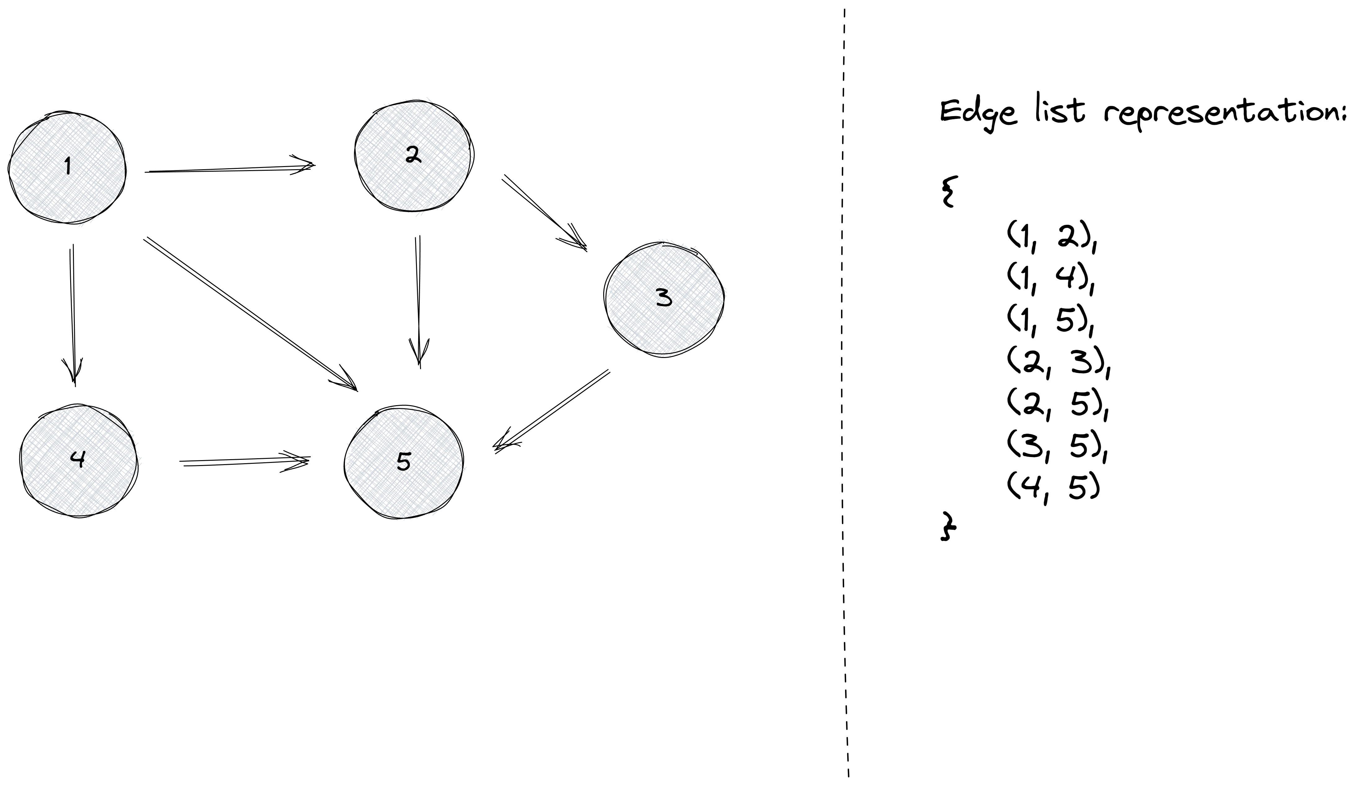
Notice that this graph is directed. If the pair (x, y) is present in the list, there is an edge starting in x and ending in y, but the opposite does not hold unless the pair (y, x) also appears in the list.

If the graph is undirected, then the edge list representation will contain the ordered pairs (x, y) and (y, x) for every pair of adjacent nodes x and y.

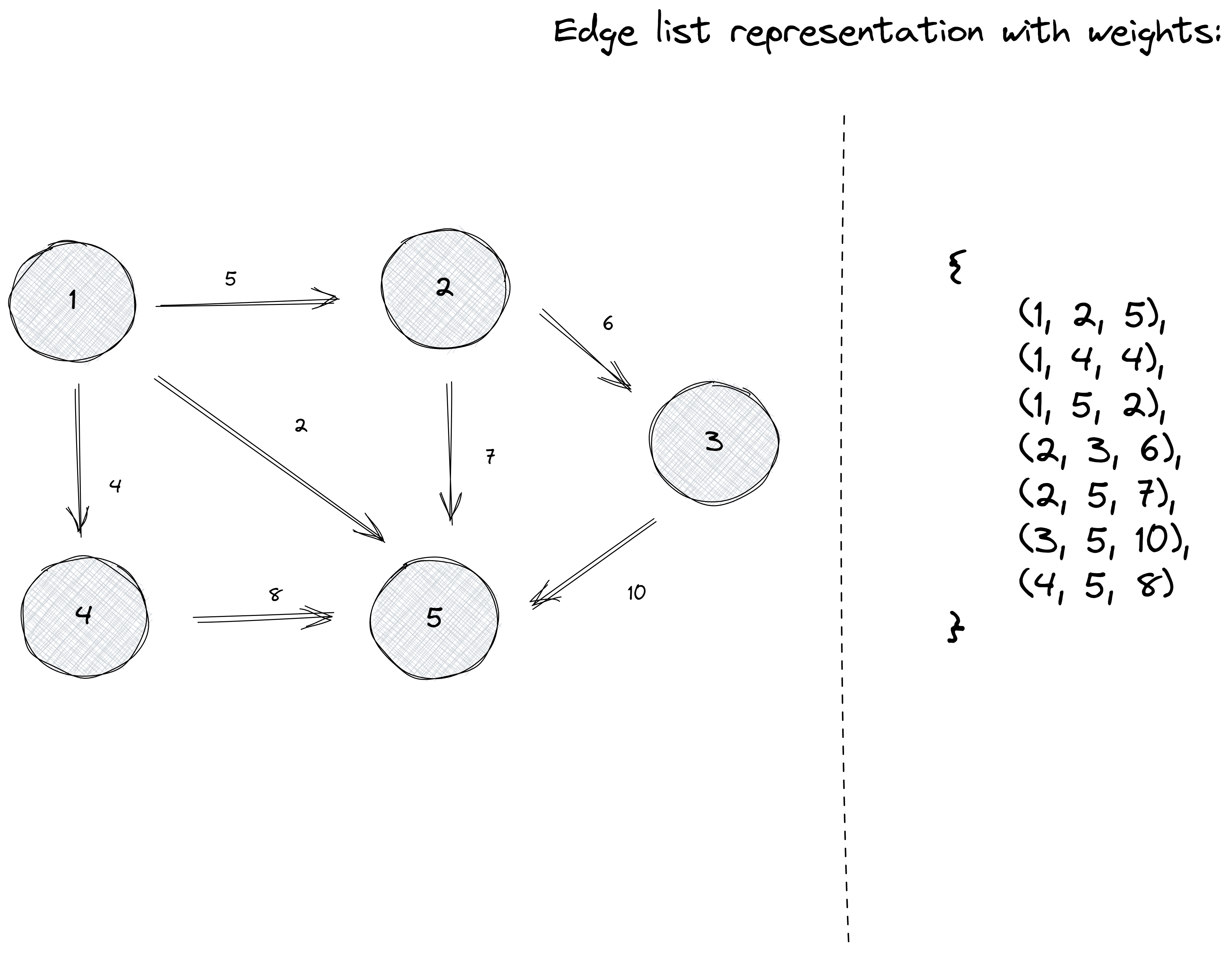
If we would like to represent a weighted graph, the most natural way to do it is by extending our representation of an edge to be a triplet instead of a pair.

Let’s say we have edges starting from node x, ending in node y, with a weight of w. One way to represent those edges would be with a triplet of the form (x, y, w).

Let’s add some weights to our previous graphs and see what its edge list representation would look like:

The edge list representation is particularly useful for algorithms that process the edges of the graphs in some order. We will be exploring some of those algorithms when dealing with the Minimum Spanning Tree or the Dynamic Connectivity problems.

But this will be in future posts. In the meantime, let’s move on to the next representation.

Adjacency Matrix

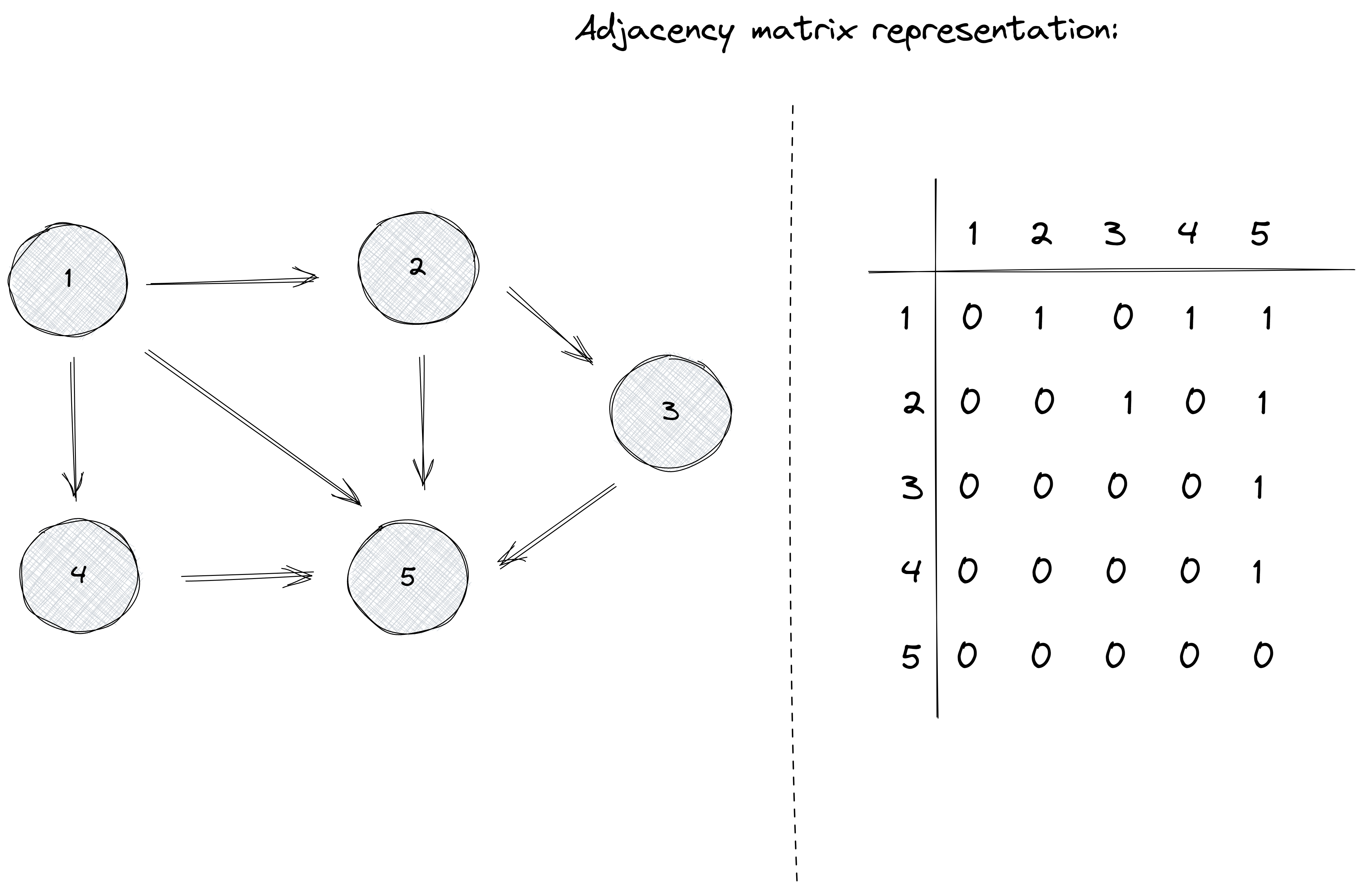
An adjacency matrix is a two-dimensional array that indicates which edges the graph contains. Let’s denote this matrix as G.

Each value G[x][y] indicates whether the graph contains an edge from node x to node y. If the edge is included in the graph, then G[x][y] = 1, and otherwise G[x][y] = 0.

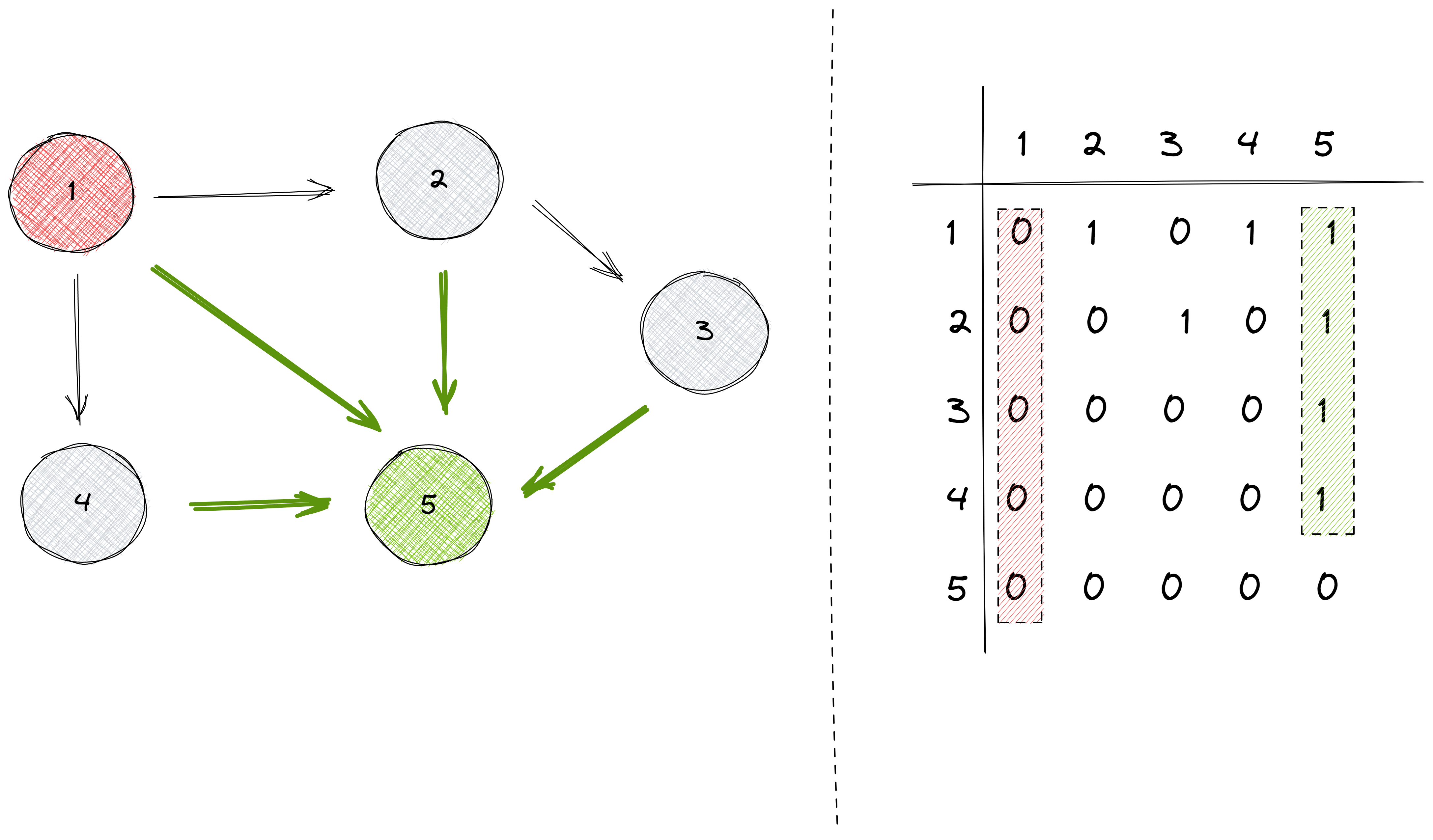
Let’s take a look at our initial graph and its corresponding adjacency matrix:

Being able to read an adjacency matrix can give you insightful information about the graph.

For example, inspecting the previous matrix, we can realize that node number 1 has the most outgoing edges, while node number 5 has the least (actually it doesn’t have any):

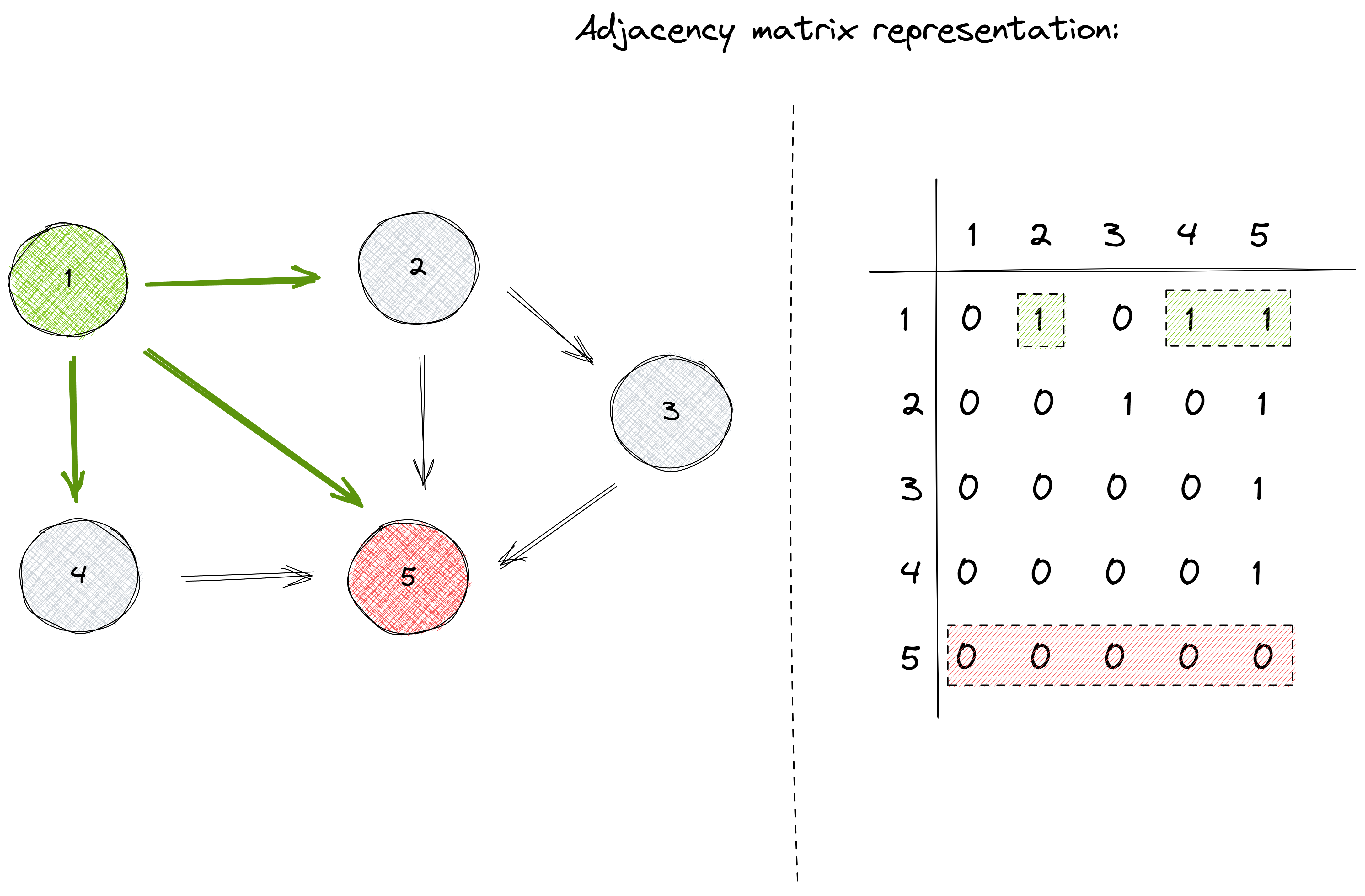
Also, we can notice how even if it doesn’t have any outgoing edge, node number 5 has the largest number of incoming edges. On the other hand, node number 1 has no incoming edges:

If the graph is weighted, the adjacency matrix representation can be extended so that the matrix contains the weight of the edge if the edge exists. Otherwise, it will contain the number 0:

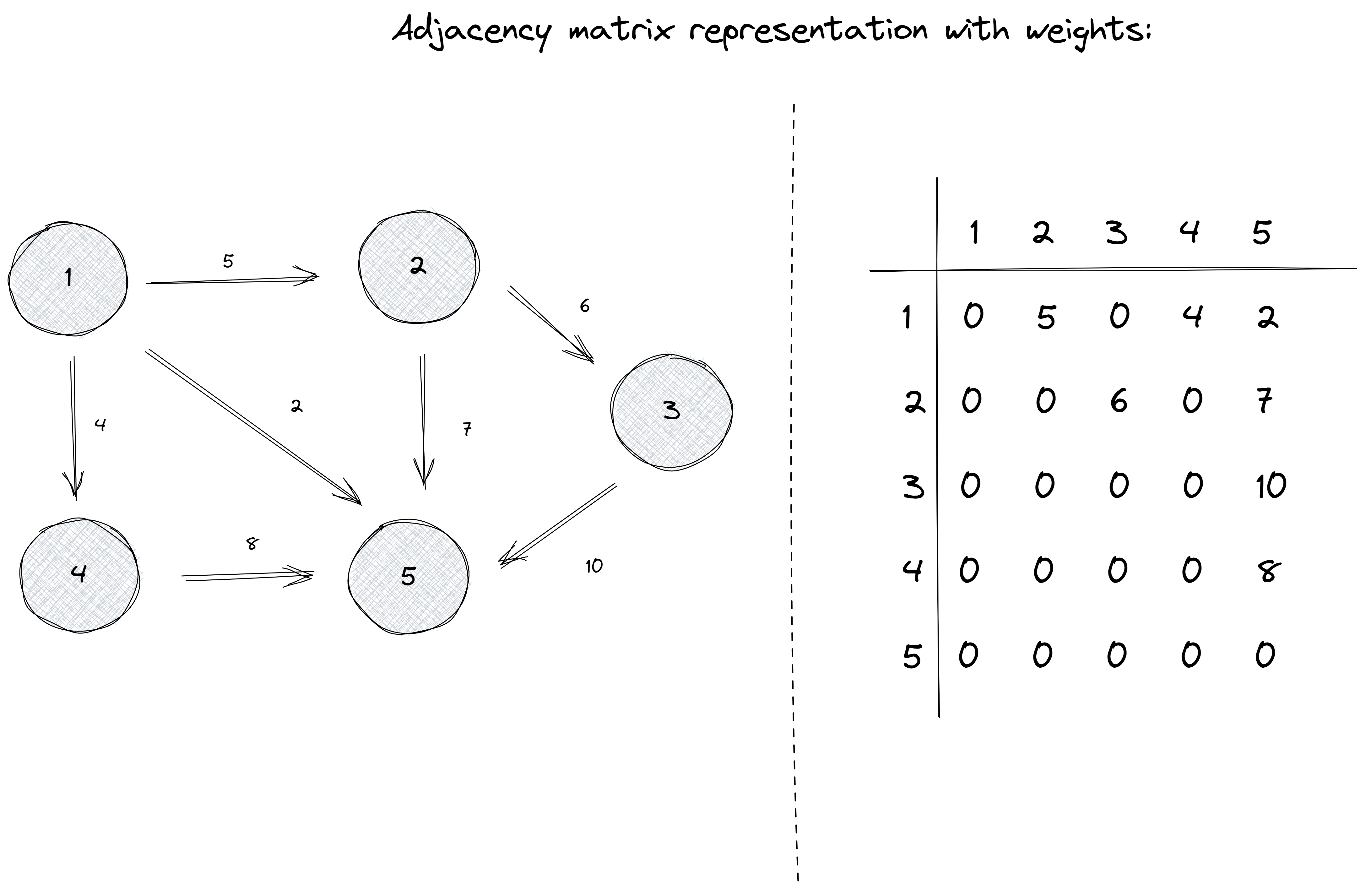
Note: We are choosing the number 0 to represent the absence of an edge because it is convenient in this case. Nevertheless, for solving some graph-related problems, this number can vary. For example, -1 or a very big (or small) number can be used instead.

One of the greatest advantages of the adjacency matrix representation is that we can efficiently verify the existence of an edge. By indexing in a position [x][y], we immediately know whether there is an edge or not between nodes x and y.

On the other hand, one of its greatest drawbacks is the fact that it requires O(n^2) space to represent a graph with n nodes.

Let’s move forward to the last representation we’ll be exploring today!

Adjacency List

The adjacency list representation is the most common way to represent graphs since most of the classic graph algorithms can be implemented very efficiently using this representation.

Every node x will be assigned a list that will contain all the nodes to which there is an edge from x.

Let’s see an example:

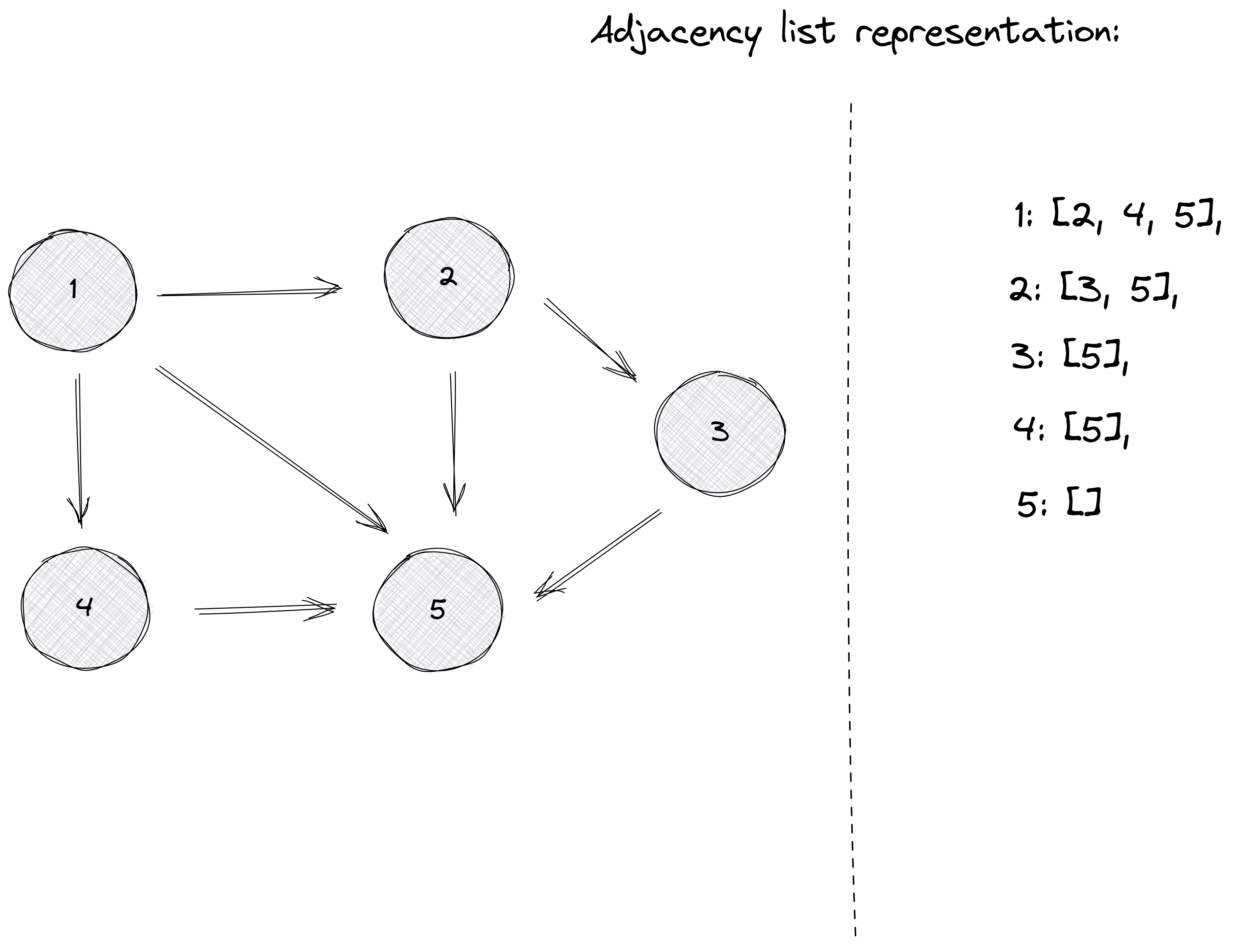
Notice how in this representation we store the exact neighbors for every node, instead of allocating space for all of the n nodes of the graph, as in the adjacency matrix representation.

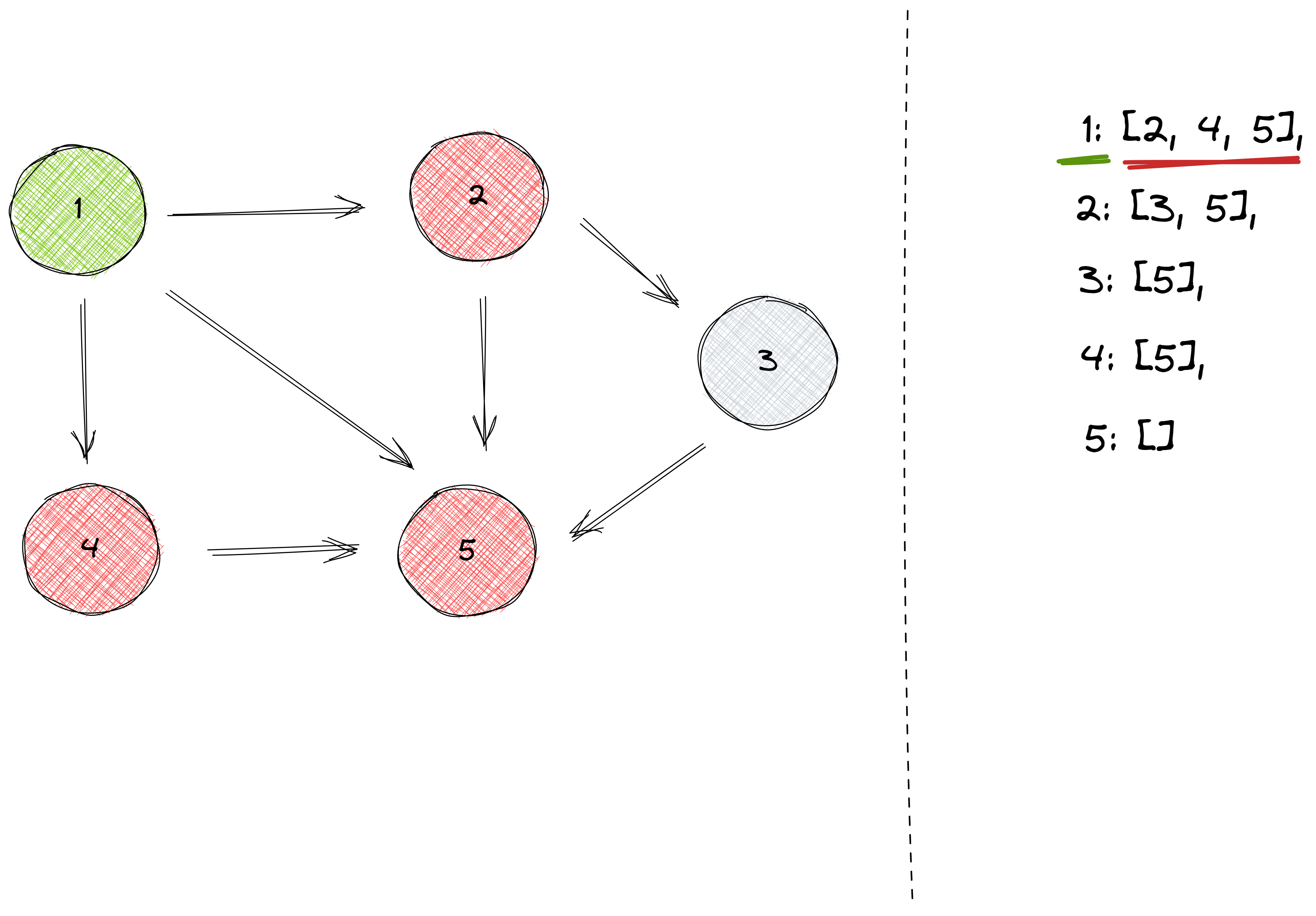
Let’s take a look at node number 1 and its neighbors:

We could store ordered pairs instead of single integers to represent weighted graphs. The pairs would be of the form (y, w), where y represents a node and w represents the weight of the edge.

Adding some weights to our previous graph:

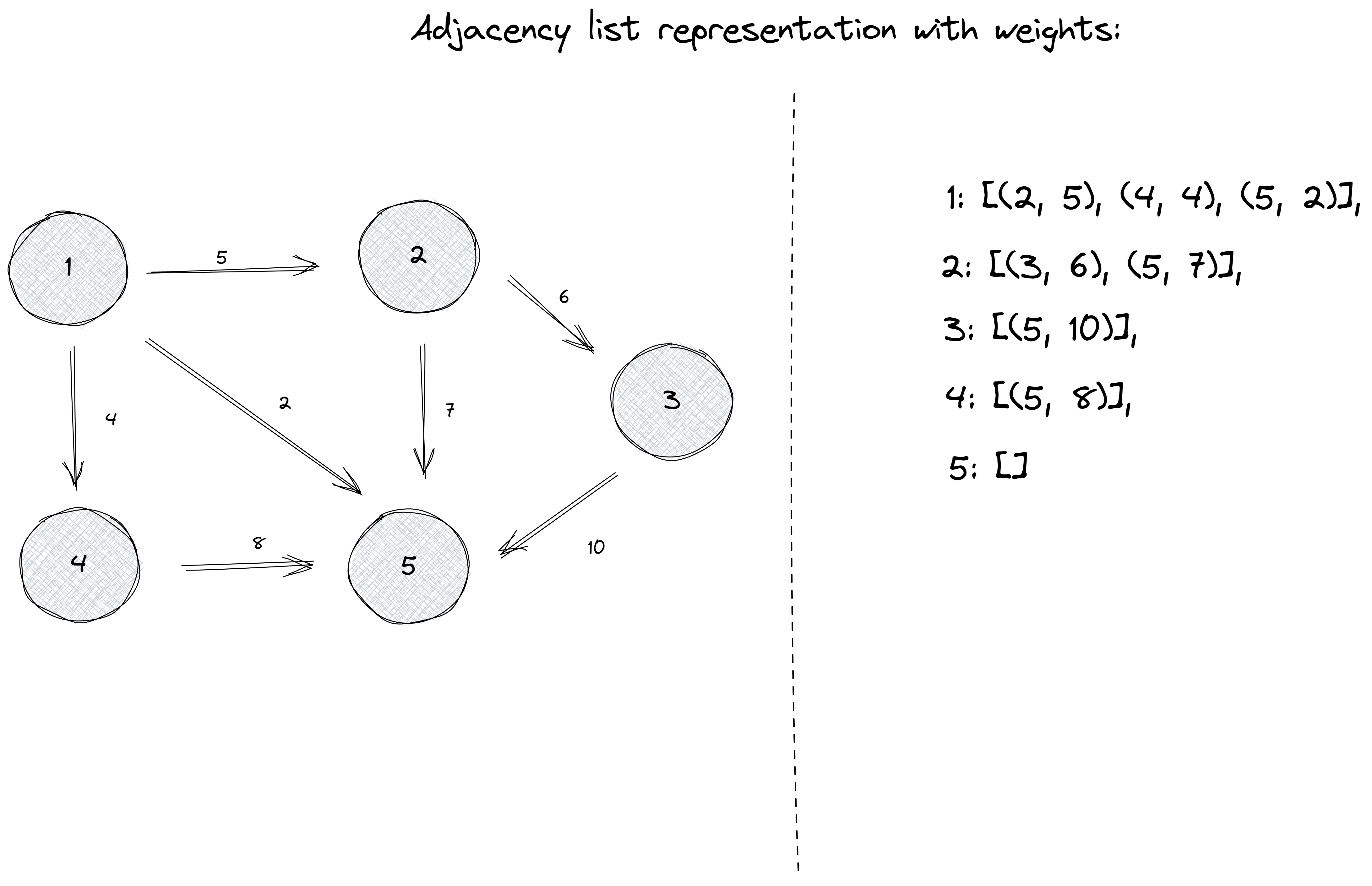
And once again, taking node number 1 as an example:

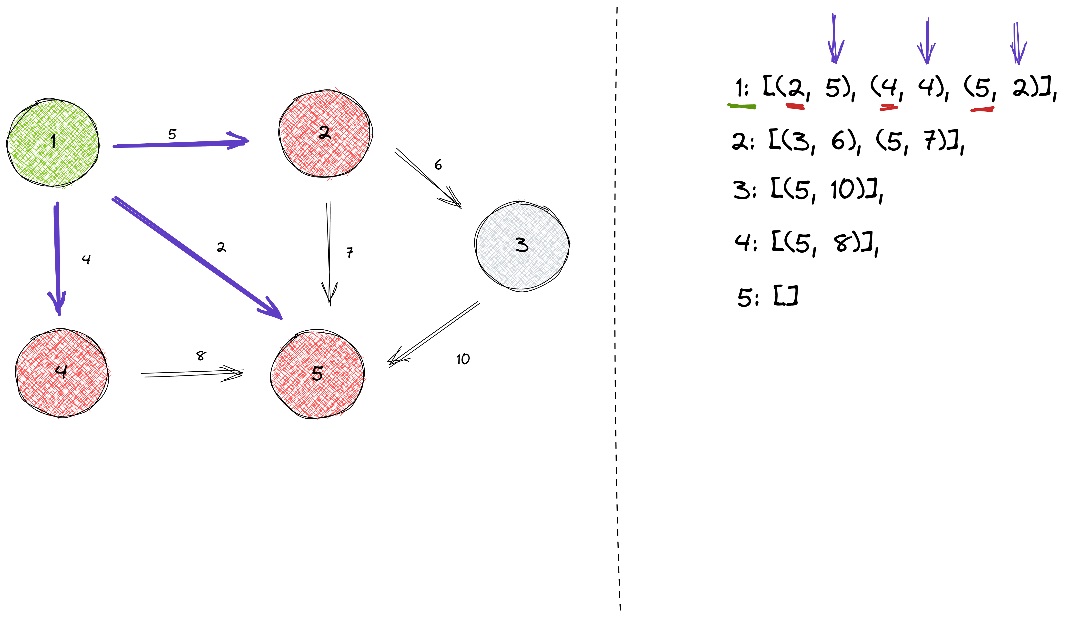
An advantage of using adjacency lists is efficiently finding the nodes to which there is an edge from a given node.

Notice that, potentially, a graph can have O(n^2) edges, which would result in this representation using the same amount of memory that the adjacency matrix representation uses. But this is rarely the case in most practical graph problems.

On the other hand, if we would want to check whether there is an edge between nodes x and y we would have to iterate the adjacency list of x until we find node y or reach the end of the list. So, adjacency matrices take the lead here.

In future posts, we will explore algorithms for traversing graphs, finding shortest paths, or determining valid colorings.

Most of these algorithms behave very differently depending on the type of representation we use for our graphs.

We have very exciting weeks ahead!

Conclusions

I hope I was able to keep igniting your passion for Graph Theory by showing you how to represent them in a computer program.

Choosing the correct representation plays an important role in solving problems that are modeled using graphs. And sometimes, the best approach is to use a combination of them.

Some takeaways:

• We have mainly three ways of representing graphs in a computer program: edge lists, adjacency matrices, and adjacency lists.

• Edge lists are useful for implementing algorithms that process the edges of the graph in a given order.

• Adjacency matrices are a very visual way of representing graphs. It allows for checking the existence of edges in constant time, but they always use O(n^2) memory for a graph of n nodes.

• Adjacency lists are the most common way of representing graphs and the preferred representation for most of the classic graph algorithms we will be exploring.

I wish you good luck when solving this week’s challenges. Don’t forget to share your progress with the community!

And if you think this post can be helpful for someone, share it with them. Nothing will make me happier!

See you next week!

---

👋 Hello, I'm Alberto, Software Developer at doWhile, Competitive Programmer, Teacher, and Fitness Enthusiast.

🧡 If you liked this article, consider sharing it.

🔗 All links | Twitter | LinkedIn